Power Analyses

library(BayesFactor)
library(brms)
library(broom)
library(ggplot2)
library(knitr)
library(magrittr)
library(tidyverse)

Background

Using data simulation, we run a power analysis for a study on how design characteristics of online platforms affect online political participation. In the study, people use a social networking site (discord) on which they discuss political matters. Participants will communicate in groups of 20 people each. This number is fixed for theory-related reasons, as we are interested in medium scale group communication. The dependent variable is how much people discuss (measured via number of opinion expressions). We’re interested how different SNS designs affect communication.

The study design is as follows:

• The website is experimentally manipulated (2 x 2 design).
  • First, the persistence of the comments is manipulated (permanent vs. ephemeral);
  • Second, the anonymity of the users is manipulated (identifiable vs. anonymous);
• To increase generalizability, the groups will discuss one of three topics: corona politics, environment, gender.
• All is between-person

So these are 2 (anonymity) x 2 (persistence) experimental factors and a 3-way generalization factor (topic), resulting in a minimum of 12 groups. Hence, the minimum sample size 12 x 20 = 240 participants.

To calculate power, the question now is how often do we need to repeat this design to achieve sufficient power? Once, twice, thrice, etc? Hence, the factor to change/affect power is repetition, ranging from 1 to 5. Note that financing would only allow 4 repetitions, so the fifth is out of curiosity.

We are simulating data which we then analyze. The data simulation is somewhat rudimentary.

• In reality, the data are nested: in groups (some groups are more active than others) and topics (some topics elicit more comments than others). Because we are lacking information on the covariance structure, we did not implement the data’s nested structure into our power analyses. We also did not analyze the data using mixed effects models, which account for nested/hierarchical structure.
• We build our simulation on standardized data. We do so, as we’re lacking the necessary information on effects sizes and variances in absolute terms.
• Opposed to what we model here, our outcome variable will not be normally distributed. Several participants will likely not express their opinions, whereas some might do so quite actively. As a result, we will analyze the data using Bayesian models modeling the outcome variable with a zero-inflated poisson distribution.

In conclusion, in our paper we will analyze the data using (Bayesian) mixed effects modeling using lme4 and/or brms.

Custom functions

Generate design

generate_design <- function(groupsize, 
                            persis, 
                            anon, 
                            topics, 
                            repetition, 
                            ...){
  
  # function generates underlying (empty) datastructure
  
  # count number of groups
  groups <- persis * anon * topics * repetition
  
  # make datastructure
  expand.grid(
    participant = 1:groupsize, 
    persistence = 1:persis - 1, # -1 to make binary
    anonymity = 1:anon - 1, 
    topic = 1:topics,
    repetition = 1:repetition) %>% 
    as.data.frame() %>% 
    rownames_to_column("id") %>% 
    mutate(
      group = rep(c(1:groups), each = groupsize))
}

Simulate data

sim_d <- function(d_frame, 
                  seed, # make results reproducible
                  effects, # vector of effects we anticipate
                  sd, 
                  groupsize, 
                  ...){
  
  # function to simulate data

  # set.seed(seed)  # uncomment to make results reproducible
  
  # compute how many participants per cell (exp. condition)
  n_cell <- groupsize_n * topics_n * repetition_n
  
  # create the DV. 
  # For now, this will be standardized, bc. of lack of concrete data
  d_frame$expressions <- NA # create variable that'll be filled next
  
  # run loop creating DVs
  for(i in 1 : repetition_n){
    for(j in 1 : topics_n){
      d_frame[d_frame$persistence == 0 & 
              d_frame$anonymity == 0 & 
              d_frame$repetition == i & 
              d_frame$topic == j, ]$expressions <- 
        rnorm(groupsize_n, effects["pers0_anon_0_m"], sd)
      d_frame[d_frame$persistence == 1 & 
              d_frame$anonymity == 0 & 
              d_frame$repetition == i & 
              d_frame$topic == j, ]$expressions <- 
        rnorm(groupsize_n, effects["pers1_anon_0_m"], sd)
      d_frame[d_frame$persistence == 0 & 
              d_frame$anonymity == 1 & 
              d_frame$repetition == i & 
              d_frame$topic == j, ]$expressions <- 
        rnorm(groupsize_n, effects["pers0_anon_1_m"], sd)
      d_frame[d_frame$persistence == 1 & 
              d_frame$anonymity == 1 & 
              d_frame$repetition == i & 
              d_frame$topic == j, ]$expressions <- 
        rnorm(groupsize_n, effects["pers1_anon_1_m"], sd)
    }
  }
  return(d_frame)
}

Analyze data

analyze_d <- function(object, approach, ...) {

  # function to analyze data and to extract results
  
  # get means
  means <- group_by(object, persistence, anonymity) %>% 
    summarize(mean = mean(expressions), .groups = 'drop')
  
  results <- data.frame(
    reps = repetition_n,
    n = nrow(object), 
    per0_anon0_m = filter(means, persistence == 0, anonymity == 0)$mean,
    per0_anon1_m = filter(means, persistence == 0, anonymity == 1)$mean,
    per1_anon0_m = filter(means, persistence == 1, anonymity == 0)$mean,
    per1_anon1_m = filter(means, persistence == 1, anonymity == 1)$mean
  )

  
    # get estimates from regression
    fit <- lm(expressions ~ persistence + anonymity, object)
    fit_rslt <- tidy(fit)
  
    # combine result
    results <- cbind(
      results,
      persistence_est = fit_rslt[fit_rslt$term == "persistence",]$estimate,
      persistence_p = fit_rslt[fit_rslt$term == "persistence",]$p.value,
      anonymity_est = fit_rslt[fit_rslt$term == "anonymity",]$estimate,
      anonymity_p = fit_rslt[fit_rslt$term == "anonymity",]$p.value
    )
  return(results)
}

Design and simulate

des_sim_fit <- function(...){
  
  # function to report and extract results
  
  d_frame <- generate_design(...)
  d <- sim_d(d_frame, ...)
  analyze_d(d, ...)
}

Estimate power

est_pow <- function(sims_n, approach, ...){
  # function to run analyse sims_n times

  tibble(sim = 1:sims_n) %>% 
  mutate(
    effect = map(sim, 
                 des_sim_fit, 
                 groupsize = groupsize_n, 
                 persis = persis_n, 
                 anon = anon_n, 
                 topics = topics_n, 
                 repetition = repetition_n, 
                 effects = effects_est, 
                 sd = sd_est,
                 approach = approach)
    ) %>%
  unnest(effect) %>%
  as.data.frame()
}

Study design

# study design
groupsize_n   <- 20
persis_n      <- 2
anon_n       <- 2 
topics_n      <- 3

# minimum sample size
sample_size <- groupsize_n * persis_n * anon_n * topics_n

We define our study design as follows:

• 20 participants per group
• 2 persistence conditions
• 2 anonymity conditions
• 3 different topics to be discussed
• 240 minimum sample size

Define effect size

We then need to define likely effects. Problem is, we don’t have good estimates of actual, raw date. To simplify, we assume normal distribution, a mean of zero and a standard deviation of one. We can hence think of effects in terms of Cohen’s d: .2 = small, .5 = medium, and .8 = large.

	persistent	ephemeral
identifiable	-.40	-.20
anonymous	-.20	0

This should lead to a main effect of persistence of d = -.20 and a main effect of anonymity of d = +.20.

pers0_anon_0_m <- -0.2
pers0_anon_1_m <-  0.0
pers1_anon_0_m <- -0.4
pers1_anon_1_m <- -0.2
effects_est <- c(pers0_anon_0_m, pers0_anon_1_m, pers1_anon_0_m, pers1_anon_1_m)
names(effects_est) <- c("pers0_anon_0_m", "pers0_anon_1_m", "pers1_anon_0_m", "pers1_anon_1_m")
sd_est <- 1

Test run

To see if our functions work, let’s make a test run with four repetitions.

repetition_n <- 4

Set-up

We first create an empty data frame, in which we will then later simulate the data.

# create design frame
d_frame <- generate_design(
  groupsize  = groupsize_n,
  persis     = persis_n,  
  anon      = anon_n,     
  topics     = topics_n,  
  repetition = repetition_n
  )
d_frame

Check if data-frame is alright.

xtabs(~persistence + anonymity + topic + repetition, d_frame)

, , topic = 1, repetition = 1

           anonymity
persistence  0  1
          0 20 20
          1 20 20

, , topic = 2, repetition = 1

           anonymity
persistence  0  1
          0 20 20
          1 20 20

, , topic = 3, repetition = 1

           anonymity
persistence  0  1
          0 20 20
          1 20 20

, , topic = 1, repetition = 2

           anonymity
persistence  0  1
          0 20 20
          1 20 20

, , topic = 2, repetition = 2

           anonymity
persistence  0  1
          0 20 20
          1 20 20

, , topic = 3, repetition = 2

           anonymity
persistence  0  1
          0 20 20
          1 20 20

, , topic = 1, repetition = 3

           anonymity
persistence  0  1
          0 20 20
          1 20 20

, , topic = 2, repetition = 3

           anonymity
persistence  0  1
          0 20 20
          1 20 20

, , topic = 3, repetition = 3

           anonymity
persistence  0  1
          0 20 20
          1 20 20

, , topic = 1, repetition = 4

           anonymity
persistence  0  1
          0 20 20
          1 20 20

, , topic = 2, repetition = 4

           anonymity
persistence  0  1
          0 20 20
          1 20 20

, , topic = 3, repetition = 4

           anonymity
persistence  0  1
          0 20 20
          1 20 20

Allocation of participants to experimental groups worked just fine.

Simulate data

Let’s create a single data-set and analyze it.

d <- sim_d(d_frame, seed = 1, effects_est, sd_est, groupsize_n)
write.csv(d, "data/data_simulated.csv") # save data.

Analyse data

Let’s check if means were created alright:

d %>% 
  group_by(persistence, anonymity) %>% 
  summarize(mean = mean(expressions), .groups = 'drop') %>% 
  kable()

persistence	anonymity	mean
0	0	-0.1460706
0	1	-0.0326302
1	0	-0.4490249
1	1	-0.1929650

Sample size small and single study, but general tendency seems to be alright.

Let’s also quickly run a regression.

fit <- lm(expressions ~ persistence + anonymity, d)
summary(fit)

Call:
lm(formula = expressions ~ persistence + anonymity, data = d)

Residuals:
    Min      1Q  Median      3Q     Max 
-3.0111 -0.6753 -0.0290  0.6915  3.7920 

Coefficients:
            Estimate Std. Error t value Pr(>|t|)    
(Intercept) -0.18173    0.05775  -3.147 0.001701 ** 
persistence -0.23164    0.06668  -3.474 0.000536 ***
anonymity    0.18475    0.06668   2.771 0.005702 ** 
---
Signif. codes:  0 '***' 0.001 '**' 0.01 '*' 0.05 '.' 0.1 ' ' 1

Residual standard error: 1.033 on 957 degrees of freedom
Multiple R-squared:  0.02022,   Adjusted R-squared:  0.01817 
F-statistic: 9.873 on 2 and 957 DF,  p-value: 5.702e-05

Results look reasonable. Both persistence and anonymity reduce disclosure.

Power analysis

Set-Up

n_sim <- 1000
n_reps <- 5

We simulate 1000 data sets for the power analyses. Up to 5 times will the set-up be repeated.

Small effects

Run analyses

Let’s next run our actual power analysis, using the effect sizes defined above (small standardized effects).

We run a power analysis with 1000 simulations per design. We test 5 designs, that is 1 to 5 repetitions.

# create empy data frame
columns <- c("sim", "reps", "per0_anon0_m", "per0_anon1_m", 
             "per1_anon0_m", "per1_anon1_m", "persistence_est", 
             "persistence_p", "anonymity_est", "anonymity_p", "n")
sims_freq_s <- data.frame(matrix(nrow = 0, ncol = length(columns))) 
colnames(sims_freq_s) = columns

t1 <- Sys.time()
for(i in 1 : n_reps){
  repetition_n  <- i
  sims_freq_s <- rbind(sims_freq_s, est_pow(approach = "frequentist", sims_n = n_sim))
}
t2 <- Sys.time()
t2 - t1

Time difference of 30.5522 secs

Visualization

Let’s inspect the results. First persistence:

ggplot(sims_freq_s) +
  geom_point(aes(sim, persistence_est, color = persistence_p < .05), 
             size = .2, alpha = .5) + 
  scale_color_manual(values = c("darkgrey", "blue")) +
  facet_wrap(facets = "reps", nrow = 1) +
  labs(color = "significant")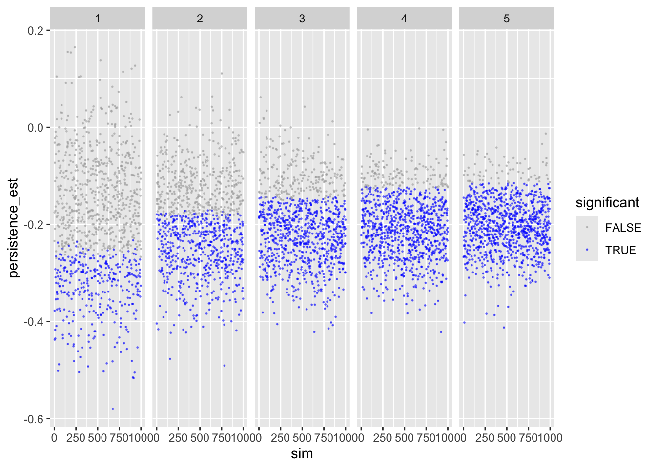

Shows that with more repetitions, effect size move closer to actual population value.

To make sure, let’s next check anonymity – should provide identical results.

ggplot(sims_freq_s) +
  geom_point(aes(sim, anonymity_est, color = anonymity_p < .05), 
             size = .2, alpha = .5) + 
  scale_color_manual(values = c("darkgrey", "blue")) +
  facet_wrap(facets = "reps", nrow = 1) +
  labs(color = "significant")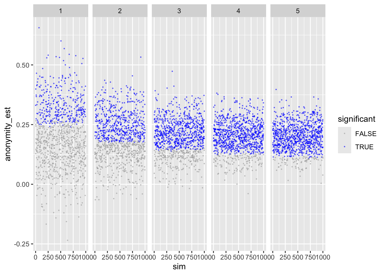

Looks good.

Cell means & main effects

Next, we compute the average means in the four cells averaged across simulations, plus the two main effects. This is more of a sanity check to see if our population values can be reproduced.

sims_freq_s %>% 
  group_by(reps) %>% 
  summarise(per0_anon0 = mean(per0_anon0_m),
            per0_anon1 = mean(per0_anon1_m),
            per1_anon0 = mean(per1_anon0_m),
            per1_anon1 = mean(per1_anon1_m),
            persistence = mean(persistence_est), 
            anonymity = mean(anonymity_est)
            ) %>% 
  as.data.frame() %>% 
  kable()

reps	per0_anon0	per0_anon1	per1_anon0	per1_anon1	persistence	anonymity
1	-0.2036146	0.0005666	-0.3999596	-0.1994476	-0.1981796	0.2023466
2	-0.1989367	-0.0033509	-0.3990509	-0.2003664	-0.1985648	0.1971352
3	-0.1990174	0.0010106	-0.3973053	-0.2033331	-0.2013158	0.1970001
4	-0.1976968	-0.0017485	-0.3996051	-0.2018917	-0.2010258	0.1968309
5	-0.1963275	-0.0035055	-0.3982119	-0.2004496	-0.1994143	0.1952921

Shows that the means resemble those we defined a priori. Same for main effects.

Power estimates

Now, let’s compute power for each number of replication.

power_freq_s <- sims_freq_s %>% 
  group_by(reps) %>% 
  summarise(n = max(n),
            persistence = sum(persistence_p < .05 & persistence_est < 0) / n_sim,
            anonymity = sum(anonymity_p < .05 & anonymity_est > 0) / n_sim)
kable(power_freq_s)

reps	n	persistence	anonymity
1	240	0.335	0.344
2	480	0.584	0.569
3	720	0.771	0.758
4	960	0.864	0.866
5	1200	0.934	0.917

dat_fr_s <- pivot_longer(power_freq_s, c(-reps, -n), names_to = "manipulation", values_to = "effect")
power_fig <- ggplot(dat_fr_s, aes(reps, effect, color = manipulation)) +
  geom_point(alpha = .9) +
  scale_x_discrete(limits = c(1:n_reps))
power_fig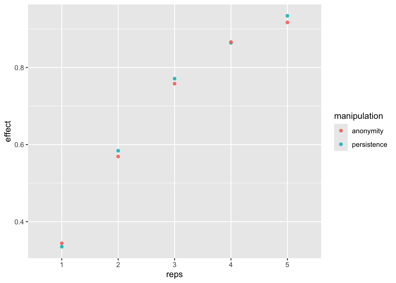

If we replicate the study at least 5 times, then we get more than 80% power.

Small-to-medium effects

Let’s next rerun our power analysis, using slightly larger effect sized (small to medium).

pers0_anon_0_m <- -0.35
pers0_anon_1_m <-  0.00
pers1_anon_0_m <- -0.70
pers1_anon_1_m <- -0.35
effects_est <- c(pers0_anon_0_m, pers0_anon_1_m, pers1_anon_0_m, pers1_anon_1_m)
names(effects_est) <- c("pers0_anon_0_m", "pers0_anon_1_m", "pers1_anon_0_m", "pers1_anon_1_m")
sd_est <- 1

Run analyses

Everything as above, but now assuming larger effects.

# create empy data frame
columns <- c("sim", "reps", "per0_anon0_m", "per0_anon1_m", 
             "per1_anon0_m", "per1_anon1_m", "persistence_est", 
             "persistence_p", "anonymity_est", "anonymity_p", "n")
sims_freq_sm <- data.frame(matrix(nrow = 0, ncol = length(columns))) 
colnames(sims_freq_sm) = columns

t1 <- Sys.time()
for(i in 1 : n_reps){
  repetition_n  <- i
  sims_freq_sm <- rbind(sims_freq_sm, est_pow(approach = "frequentist", sims_n = n_sim))
}
t2 <- Sys.time()
t2 - t1

Visualization

Let’s inspect the results. First persistence:

ggplot(sims_freq_sm) +
  geom_point(aes(sim, persistence_est, color = persistence_p < .05), 
             size = .2, alpha = .5) + 
  scale_color_manual(values = c("darkgrey", "blue")) +
  facet_wrap(facets = "reps", nrow = 1) +
  labs(color = "significant")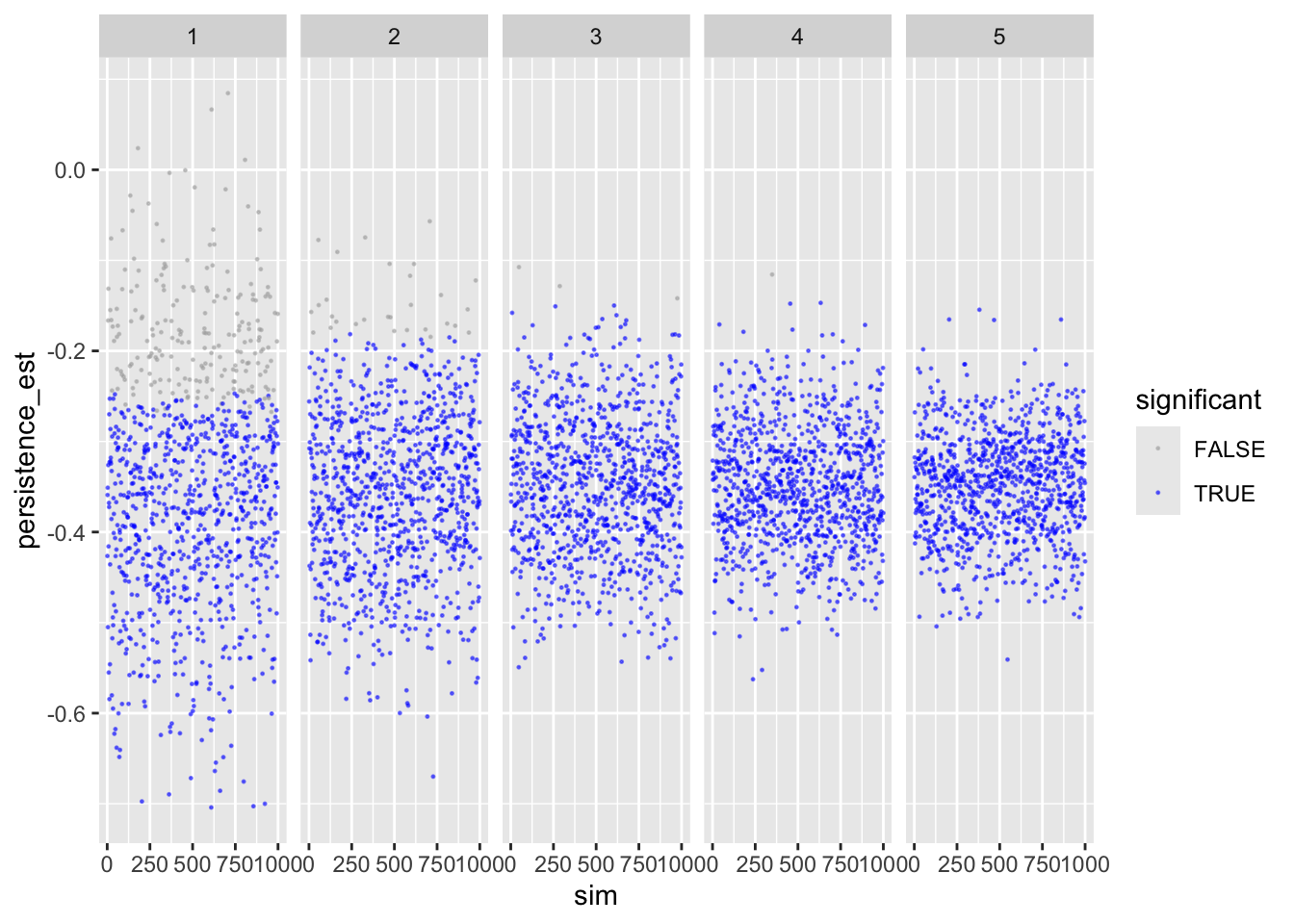

Shows that with more repetitions, effect size moves closer to actual population value.

To make sure, let’s next check anonymity – should provide identical results.

ggplot(sims_freq_sm) +
  geom_point(aes(sim, anonymity_est, color = anonymity_p < .05), 
             size = .2, alpha = .5) + 
  scale_color_manual(values = c("darkgrey", "blue")) +
  facet_wrap(facets = "reps", nrow = 1) +
  labs(color = "significant")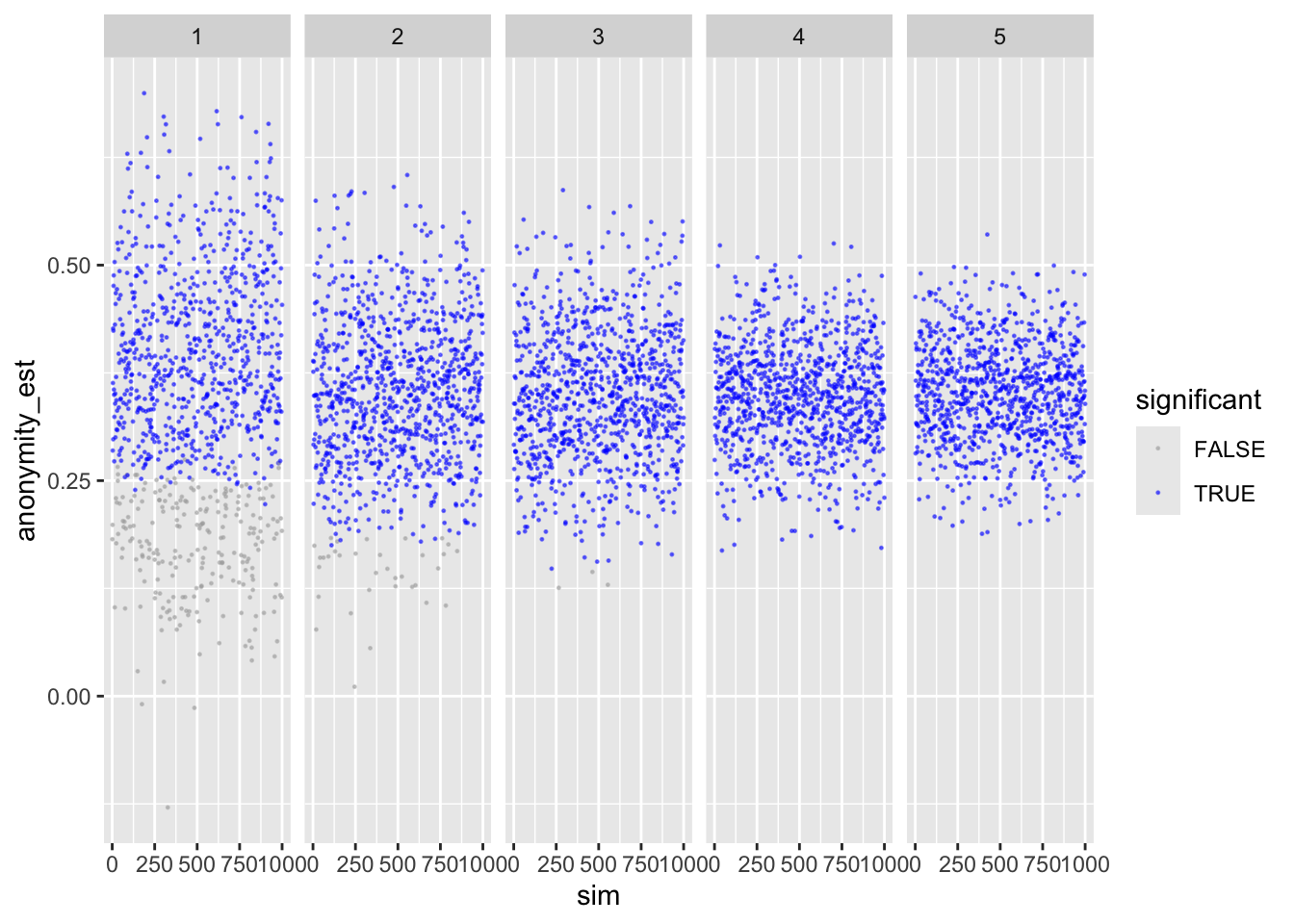

Looks good.

Cell means & main effects

Next, we compute the average means in the four cells averaged across simulations, plus the two main effects. This is more of a sanity check to see if our population values can be reproduced.

sims_freq_sm %>% 
  group_by(reps) %>% 
  summarise(per0_anon0 = mean(per0_anon0_m),
            per0_anon1 = mean(per0_anon1_m),
            per1_anon0 = mean(per1_anon0_m),
            per1_anon1 = mean(per1_anon1_m),
            persistence = mean(persistence_est), 
            anonymity = mean(anonymity_est)
            ) %>% 
  kable()

reps	per0_anon0	per0_anon1	per1_anon0	per1_anon1	persistence	anonymity
1	-0.3529767	0.0016533	-0.7008929	-0.3525972	-0.3510833	0.3514628
2	-0.3488914	0.0030501	-0.6995804	-0.3545085	-0.3541238	0.3485067
3	-0.3504833	0.0010607	-0.6964101	-0.3487588	-0.3478731	0.3495976
4	-0.3494230	-0.0014467	-0.6983255	-0.3508370	-0.3491464	0.3477324
5	-0.3519374	0.0031855	-0.6978309	-0.3493555	-0.3492172	0.3517991

Shows that the means resemble those we defined a priori. Same for main effects.

Power estimates

Now, let’s compute power for each number of replication.

power_freq_sm <- sims_freq_sm %>% 
  group_by(reps) %>% 
  summarise(persistence = sum(persistence_p < .05 & persistence_est < 0) / n_sim,
            anonymity = sum(anonymity_p < .05 & anonymity_est > 0) / n_sim,
            n = max(n))
kable(power_freq_sm)

reps	persistence	anonymity	n
1	0.792	0.767	240
2	0.971	0.966	480
3	0.997	0.997	720
4	0.999	1.000	960
5	1.000	1.000	1200

If we replicate the study at least 3 times, then we get more than 80% power.

dat_fr_sm <- pivot_longer(power_freq_sm, c(-reps, -n), names_to = "manipulation", values_to = "effect")
power_fig <- ggplot(dat_fr_sm, aes(reps, effect, color = manipulation)) +
  geom_point(alpha = .9) +
  scale_x_discrete(limits = c(1:n_reps))
power_fig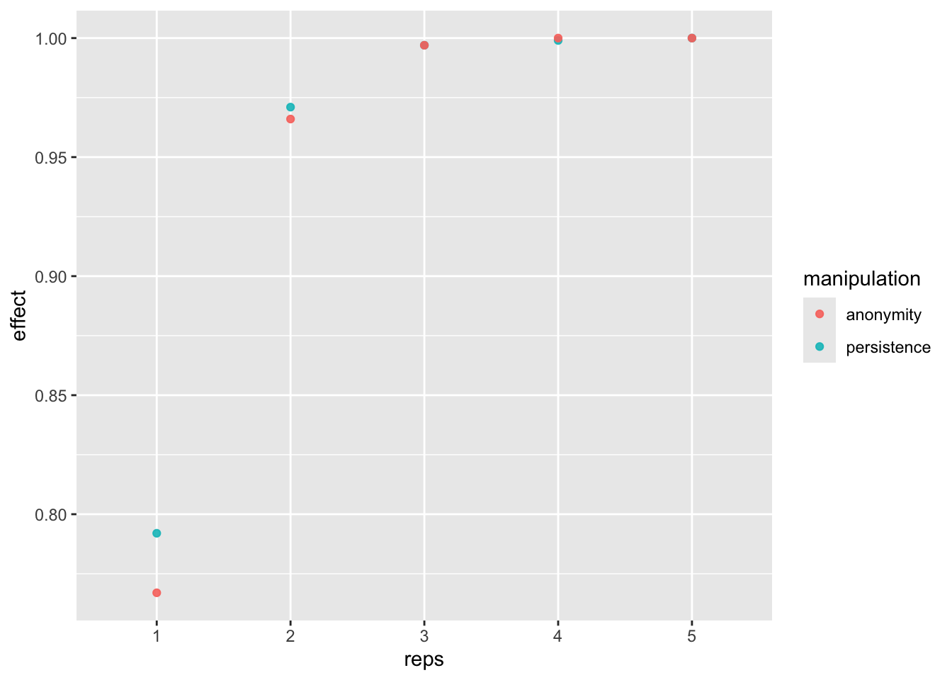

Summary

Tables

For small effects:

tab_s <- cbind(
  Replications = power_freq_s$reps,
  N = power_freq_s$n,
  pers_power = power_freq_s$persistence,
  anon_power = power_freq_s$anonymity
)
kable(tab_s)

Replications	N	pers_power	anon_power
1	240	0.335	0.344
2	480	0.584	0.569
3	720	0.771	0.758
4	960	0.864	0.866
5	1200	0.934	0.917

For small-to-medium effects

tab_sm <- cbind(
  Replications = power_freq_sm$reps,
  N = power_freq_sm$n,
  pers_power = power_freq_sm$persistence, 
  anon_power = power_freq_sm$anonymity
)
kable(tab_sm)

Replications	N	pers_power	anon_power
1	240	0.792	0.767
2	480	0.971	0.966
3	720	0.997	0.997
4	960	0.999	1.000
5	1200	1.000	1.000

Figures

# dat_bf_s <- pivot_longer(power_bf_s, c(-reps, -n), names_to = "manipulation", values_to = "effect")
# dat_bf_s$effectsize <- "small"
# dat_bf_sm <- pivot_longer(power_bf_sm, c(-reps, -n), names_to = "manipulation", values_to = "effect")
# dat_bf_sm$effectsize <- "small-to-medium"
# dat_bf <- rbind(dat_bf_s, dat_bf_sm)
# dat_bf$analysis <- "Bayes Factor > 10"
# dat_bf$manipulation <- recode(dat_bf$manipulation, `bf_pers > 10` = "persistence", `BF_anon > 10` = "anonymity")

dat_fr_s$effectsize <- "small"
dat_fr_sm$effectsize <- "small-to-medium"
dat_fr <- rbind(dat_fr_s, dat_fr_sm)
# dat_fr$analysis <- "Frequentist"

dat <- dat_fr %>% 
  rename(Manipulation = manipulation,
         `Effect size` = effectsize,
         Effect = effect,
         Replications = reps) %>% 
  mutate(
    # analysis = factor(analysis, levels = c("Frequentist", "Bayes Factor > 10")),
    `Effect size` = factor(`Effect size`, levels = c("small-to-medium", "small")))

power_fig <- ggplot(dat, aes(Replications, Effect, color = `Effect size`, shape = Manipulation)) +
  scale_color_manual(values=c("black", "grey60")) +
  geom_vline(xintercept = 4, linetype = "dashed", color = "grey") + 
  geom_point(alpha = .9) +
  scale_x_discrete(limits = c(1:n_reps))
power_fig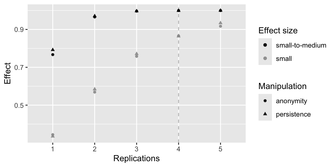

ggsave("figures/fig_power.png", width = 8, height = 4)